Introduction
Diffusion theory is the modeling of photon transport due to photon movement down concentration gradients. Diffusion theory is appropriate in medium dominated by scattering rather than absorption so that each photon undergoes many scattering events before being terminated by an absorption event. The photon has a relatively long residence time which allows the photon to engage in a random walk within the medium.
Diffusion theory = Photons falling down a gradient of photon concentration.
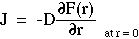
F(r,t) = cC(r,t)
Fick's 1st law of diffusion
Diffusion occurs in response to a concentration gradient expressed as the change in concentration due to a change in position,  . The local rule for movement or flux J is given by Fick's 1st law of diffusion:

 [cm2/s] and the negative gradient of concentration, [cm-3 cm-1] or [cm-4]. The negative sign indicates that J is positive when movement is down the gradient, i.e., the negative sign cancels the negative gradient along the direction of positive flux.
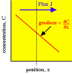
The flux J is driven by the negative gradient in the direction of increasing x.
For light, the diffusivity is proportional to the diffusion length D [cm] and the speed of light c:
where D = 1/(3 µs(1-g)). The units of velocity [cm/s] times the units of length [cm] yield the units of diffusivity [cm2/s]. The following example describes the local diffusion of red light in milk.
For optical diffusion, Fick's 1st law is expressed as the energy flux J [W cm-2] proportional to the diffusion constant D [cm] and the negative fluence gradient dF/dx:

. The local rule for movement or flux J is given by Fick's 1st law of diffusion: [cm2/s] and the negative gradient of concentration, [cm-3 cm-1] or [cm-4]. The negative sign indicates that J is positive when movement is down the gradient, i.e., the negative sign cancels the negative gradient along the direction of positive flux.The flux J is driven by the negative gradient
in the direction of increasing x.Examplearbitrary units | Consider a local concentration of 106 units per cm3 which drops by 10% over a distance of 1 cm. Then the gradient is -105 [units cm-4]. Assume the diffusivity is 103[cm2/s]. Then the flux J equals: |
For light, the diffusivity is proportional to the diffusion length D [cm] and the speed of light c:
 = cD
= cD
Exampleoptical energy | Consider a local fluence rate F of 1 W/cm2 in milk (n = 1.33, µs(1-g) = 10 cm-1).
|
For optical diffusion, Fick's 1st law is expressed as the energy flux J [W cm-2] proportional to the diffusion constant D [cm] and the negative fluence gradient dF/dx:
and substituting F/c for C. The factors c and 1/c cancel to yield the above equation.Fick's 2nd law of diffusion
Consider diffusion at the front and rear surfaces of an incremental planar volume. Fick's 2nd law of diffusion describes the rate of accumulation (or depletion) of concentration within the volume as proportional to the local curvature of the concentration gradient. The local rule for accumulation is given by Fick's 2nd law of diffusion:

 [cm-3 cm-2] or [cm-5]. The accumulation is positive when the curvature is positive, i.e., when the concentration gradient is more negative on the front end of the planar volume and less negative on the rear end so that more flux is driven into the volume at the front end than is driven out of the volume at the rear end.
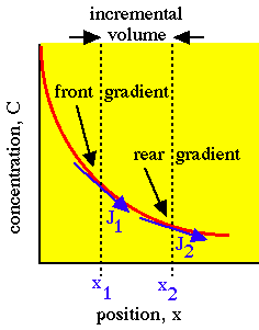
Incremental planar volume accumulates concentration because the front gradient at x 1 drives more flux J1 into the volume than the flux J2 driven out of the volume by the rear gradient at x2.
The differential equation for optical diffusion is simply Fick's 2nd law with the substitution of the product cD for the diffusivity and substitution of F/c for concentration C, although the 1/c factors introduced on both sides of the equation cancel:

[cm2/s] and the 2nd derivative (or curvature) of the concentration, [cm-3 cm-2] or [cm-5]. The accumulation is positive when the curvature is positive, i.e., when the concentration gradient is more negative on the front end of the planar volume and less negative on the rear end so that more flux is driven into the volume at the front end than is driven out of the volume at the rear end.Incremental planar volume accumulates concentration because the front gradient at x 1 drives more flux J1 into the volume than the flux J2 driven out of the volume by the rear gradient at x2.
The differential equation for optical diffusion is simply Fick's 2nd law with the substitution of the product cD for the diffusivity
and substitution of F/c for concentration C, although the 1/c factors introduced on both sides of the equation cancel:Connecting optical transport theory and Fick's 1st law of diffusion.
The early work on neutron scattering theory in nuclear reactors first developed the connection between transport theory and Fick's 1st law of diffusion. The resulting statement of diffusion is also applied to optical transport. Consider the following problem:
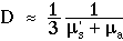
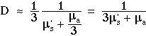
For photon transport, the term µs' = µs(1 - g) is substituted the above µs which described isotropic scattering used in the above treatment.
In summary, the connection between transport theory and Fick's 1st law of diffusion is based on the linearization of F(r) around the value F(0) and on the approximation of D by the value 1/(3 µs').
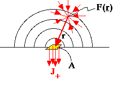 Light scattered at position r passes through a small aperture with area A contributing to the flux J+. |
- given a homogeneous isotropically scattering medium with scattering coefficient µs
- given a small aperture with area A at the origin (r = 0)
- given a fluence rate F(0) at the origin
- assume that the fluence rate F(r) at a position r near to the aperture is approximated by

- calculate the net flux through the small aperture with area A due to scattering from all the surrounding volume:
- the scattered flux at r is µsF(r) = µs( F(0) + r(dF(r)/drat r=0) ) where r is the distance from r to the origin.
- the fraction of scattered flux from r that survives a pathlength r without being scattered or absorbed is exp(-µtr), where µt = µs + µa. Consider the case of negligible absorption compared to scattering so µt = µs.
- the fraction of surviving scattered flux from r that passes through A is Acos
 /(4
/(4 r2).
r2). - integrate the flux from r over all possible and r for the hemisphere above the aperture:
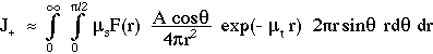
- a similar integration for the scattering from the hemisphere below the aperture yields a positive value J- for flux passing through A in the other direction opposite to J+.
- the net flux J = J+ - J-
- The final expression for the net flux J has the form of Fick's 1st law of diffusion if the diffusion constant D has the following value:
 , where
For photon transport, the term µs' = µs(1 - g) is substituted the above µs which described isotropic scattering used in the above treatment.
In summary, the connection between transport theory and Fick's 1st law of diffusion is based on the linearization of F(r) around the value F(0) and on the approximation of D by the value 1/(3 µs').
Limits of diffusion theory
There are limits to the applicability of diffusion theory.
It is important to remember that diffusion theory simply attempts to mimic Fick's 1st law of diffusion by a proper choice of D to relate J and -dF/dr. The approximation of F(r) as simply a linear perturbation of the value F(0) neglects higher order terms that depend on d2F/dr2. Sometimes the gradient has significant curvature within the spherical regime from which exp(-µs' r) allows photons to pass through the aperture. In such regions, the linear approximation to F(r) is inadequate and diffusion theory is inaccurate. Two cases of curvature deserve emphasis:
It is important to remember that diffusion theory simply attempts to mimic Fick's 1st law of diffusion by a proper choice of D to relate J and -dF/dr. The approximation of F(r) as simply a linear perturbation of the value F(0) neglects higher order terms that depend on d2F/dr2. Sometimes the gradient has significant curvature within the spherical regime from which exp(-µs' r) allows photons to pass through the aperture. In such regions, the linear approximation to F(r) is inadequate and diffusion theory is inaccurate. Two cases of curvature deserve emphasis:
Near a source
The gradients are very steep near a point source or collection of point sources with both the exponential term exp(-r/(4cDt)) and the term 1/r causing significant curvature in the gradients. Distant from sources, gradients become gradual and diffusion theory is more accurate.Absorption
Strong absorption prevents photons from engaging in an extended random walk. The approximation µt = µs' becomes inadequate. In common use is the approximation:Time-resolved Diffusion Theory
The solution to Fick's 2nd Law of diffusion for the case of a point source of energy, Uo [units], deposited at zero time (t = 0) at the origin (r = 0) is C(r,t) [units cm-3]:
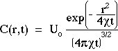
For the case of optical diffusion, let F = cC and = cD. Let the point source be an impulse of energy Uo [J]. The expression for fluence rate F(r,t) [W cm-2] becomes:
[cm2/s] is the diffusivity. In the denominator, the product t has units of [cm2] which is taken to the 3/2 power to yield units of [cm3]. The exponential in the numerator is dimensionless. The units of Uo can be the units of any extensive variable which is able to diffuse throughout a volume. Hence, C(r,t) has the proper dimensions for concentration, [units cm-3]. The above expression for C(r,t) is a solution to Fick's 2nd law of diffusion and describes spherically symmetric diffusion from a point impulse source in a homogeneous medium with no boundaries. For the case of optical diffusion, let F = cC and
= cD. Let the point source be an impulse of energy Uo [J]. The expression for fluence rate F(r,t) [W cm-2] becomes:Time-resolved diffusion Theory:
Examples
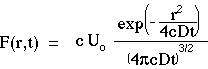
The following figures illustrate the time-resolved transport of light from an impulse isotropic point source of energy within a homogeneous unbounded medium with absorption and scattering properties.
The C program that generated the data in the above figures is listed here.
| The time-resolved fluence rate F(r,t) is plotted versus r at three timepoints: t = 5, 100, and 1000 ps. medium: µa = 1.0 cm-1, µs(1 - g) = 10.0 cm-1, nt = 1.33 impulse energy: Uo = 1 J | 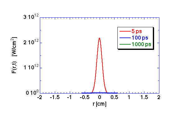 Click on figure to enlarge |
| The same data plotted as a semi-log plot. |  Click on figure to enlarge |
Steady-state Diffusion Theory
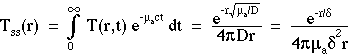
The time-resolved fluence rate F(r,t) [W/cm2] in response to an impulse of energy Uo [J] and the steady-state fluence rate Fss(r) [W/cm2] in response to an isotropic point source of continuous power Po [W] are summarized:
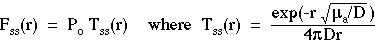
where the transport factors T(r,t) [cm-2 s-1] and Tss(r) [cm-2] have been introduced to more carefully distinguish the source, the transport, and the fluence rate. Note on notation: In this class, we use Fss(r) rather than F(r) to especially emphasize the steady-state fluence rate from the time-resolved fluence rate. However, F(r) should be used outside this class.
The above expression for Tss(r) can be obtained by integrating T(r,t)exp(-µact) over all time to yield the total accumulated amount of photon transport to each position r. The factor exp(-µact) accounts for photon absorption (recall that ct = pathlength so this expression is simply Beer's law for photon survival) and causes photon concentration to approach zero as time goes to infinity. The expression for Tss(r) is derived:
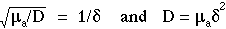
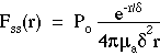
 which is the incremental distance from the source that causes Fss(r) to decrease to 1/e its initial value. The penetration depth is a parameter which is very easily understood in experimental measurements and consequently has more intuitive value to some people than D which is important from the perspective of the local step size of the diffusion process. In this class we will often use the following expression for Fss(r) when we prefer to emphasize the roles of µaand :
where the transport factors T(r,t) [cm-2 s-1] and Tss(r) [cm-2] have been introduced to more carefully distinguish the source, the transport, and the fluence rate. Note on notation: In this class, we use Fss(r) rather than F(r) to especially emphasize the steady-state fluence rate from the time-resolved fluence rate. However, F(r) should be used outside this class.
The above expression for Tss(r) can be obtained by integrating T(r,t)exp(-µact) over all time to yield the total accumulated amount of photon transport to each position r. The factor exp(-µact) accounts for photon absorption (recall that ct = pathlength so this expression is simply Beer's law for photon survival) and causes photon concentration to approach zero as time goes to infinity. The expression for Tss(r) is derived:
Steady-state diffusion Theory:
Examples
The following figures illustrate the transport of light from a steady-state isotropic point source of power within a homogeneous unbounded medium with absorption and scattering properties.
The C program that generated the data in the above figures is listed here.
| The steady-state fluence rate F(r) is plotted versus r. medium: µa = 1.0 cm-1, µs(1 - g) = 10.0 cm-1, nt = 1.33 impulse power: Po = 1 W |  Click on figure to enlarge |
| The same data plotted as a semi-log plot. | 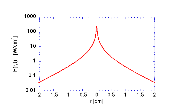 Click on figure to enlarge |
Frequency-domain Diffusion Theory:
Isotropic point source in infinite medium
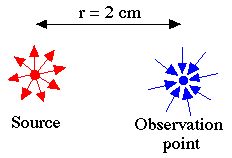
A light source may be modulated sinusoidally to yield a sinusoidally varying fluence rate distribution at a distant observation point within a medium. Such a modulated concentration will propagate in the medium and is often called a photon density wave. Consider a modulated isotropic point source of light within a homogenous turbid medium with no boundaries.
The point source S has a steady-state power So [W] which is modulated sinusoidally by a modulation factor Mosin( t), where 0 < Mo < 1:

In response to this modulated source, the modulated fluence rate F(r,t) at r is described:
The expressions for Tss(r), k" and k' are:
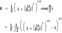
where

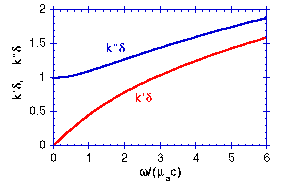
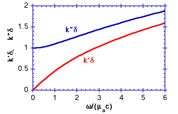
The behavior of k' and k" are shown in the following figure which plots k' and k" as functions of /(µac):
 Click figure to enlarge
The above expressions are equivalent to the expressions published by Schmitt et al. 1992 which in turn are equivalent to the expressions published by Fishkin et al. 1991,1993. Link to references..
At the observation point, the persistence of the source modulation is called the modulation, M, and is often described in the literature as (ACout/DCout)/(ACin/DCin) which equals:
 [radians], which equals:

The ratio/(µac) describes the number of radians of modulation cycle that occur in one mean photon lifetime. Only 1/e or 37% of photons survive after a time period of 1/(µac) [s]. is an angle specified by the ratio /(µac), and approaches zero for low modulation frequencies and approaches 90° at the highest modulation frequencies, >> µac.
The point source S has a steady-state power So [W] which is modulated sinusoidally by a modulation factor Mosin(
In response to this modulated source, the modulated fluence rate F(r,t) at r is described:
The expressions for Tss(r), k" and k' are:
where
The behavior of k' and k" are shown in the following figure which plots k'
 Click figure to enlarge
The above expressions are equivalent to the expressions published by Schmitt et al. 1992 which in turn are equivalent to the expressions published by Fishkin et al. 1991,1993. Link to references..
At the observation point, the persistence of the source modulation is called the modulation, M, and is often described in the literature as (ACout/DCout)/(ACin/DCin) which equals:
The ratio
- At very low modulation frequencies, << µac, there is little modulation during the lifetime of a photon. Consequently, photon migration has little impact on the transport of the modulation. The value of k" approaches one so k" approaches 1/, therefore M approaches unity. The value of k' approaches zero, therefore approaches zero. The observed modulation of Fss(r,t) mimics the source modulation with no loss of modulation and no phase lag. F(r,t) approaches the behavior SoTss(r)(1 + Mosin(t)).
- At high modulation frequencies, as the modulation frequency approaches the value of µac or greater, there is significant modulation during the lifetime of the photon. Consequently, the photon can diffuse during its lifetime and thereby smear the spatial resolution of the modulation. F(r,t) exhibits significant loss of modulation (M < 1) and an increased phase lag ( > 0): F(r,t) = SoTss(r)(1 + MoMsin(t - k'r))
Frequency-domain diffusion theory:
Examples
The following figure illustrates the time-resolved signal F(r,t) in blue and the source S(t) in red. Note the greatly decreased Fss, the slightly decreased modulation M, and the phase lag at the observation point.
The C program that generated the data in the above figure is listed here.
The following figures illustrates the modulation of the photon density wave as it propagates into the medium.
The C program that generated the data in the above figures is listed here.
 source: f = 400 MHz, So = 1 W, Mo = 1.0 medium: µa = 1.0 cm-1, µs(1 - g) = 10.0 cm-1, nt = 1.33 |  Click on figure to enlarge |
The following figures illustrates the modulation of the photon density wave as it propagates into the medium.
| The factor Msin(- Note that very large distances are needed to develop cyclic modulation due to phase lag. Photon density waves do not present multiple cycles in typical experiments. The period of one cycle is rk'/ source: f = 400 MHz, Mo = 1.0 medium: µa = 1.0 or 0.1 cm-1, µs(1 - g) = 10.0 cm-1, nt = 1.33 | 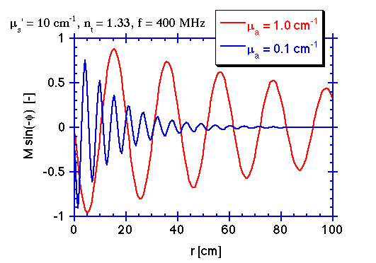 Click on figure to enlarge |
| The fluence rate F(r,t) is plotted versus position r for a specific time (t = 0 [s] or multiples of rk'/ | 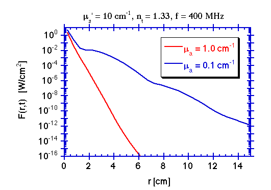 Click on figure to enlarge |
Source:http://omlc.ogi.edu/classroom/ece532/class5/fdexamples.html